materials-chemistry/ai produced the result/Scientific Reports 2025 · v2

Regression models predict how graphene loading changes aluminium's electron emission

Researchers fitted a range of machine learning regression models to existing emission measurements of aluminium and aluminium–graphene composites, then used the fitted models to produce emission curves for higher graphene contents that had not been measured.

spectrum · one line per step, placed by what the step does · bright lines used AI

Machine learning enhanced ultra-high vacuum system for predicting field emission performance in graphene reinforced aluminium based metal matrix composites
Scientific Reports, 2025

doi:10.1038/s41598-025-10946-7 · record aix-00133 v2 · checked 2026-10-09

ai-resultrole of AI

AI was for: Property prediction
Model family: Gaussian process, Support vector machine, Random forest, Gradient-boosted trees, Multilayer perceptron, Linear model
Checked by: Held-out
Code: not reported

The finding the paper is about came from the AI.

read as

The science is explained before the AI appears. Switch to field specialist to go straight to the method.

Assumes the discipline and goes straight to the method.

The diagram, the record and what the paper did not report are identical in both modes. Only the framing changes — never the evidence.

Introduction by AIxSci · plain language

What this research was about

Diagram of the synthesis process for aluminium-graphene composites at varying graphene weight percentages. — Synthesis method used to make aluminium-graphene composites at different graphene concentrations.Schematic 1 from Pradhan et al., Scientific Reports 2025 · source · CC BY · resized

Some materials release electrons from their surface when a strong electric field is applied nearby, without being heated. This is called field emission, and it matters for devices such as flat displays and electron sources. A useful material emits a usable current at a modest field. The field at which emission begins is known as the turn-on field, and a lower one is generally preferred. Aluminium on its own is a mediocre emitter, but mixing in graphene, a sheet material one atom thick, gives the surface many fine edges where the electric field concentrates. Measuring each candidate mixture is slow work: the composites must be milled, sintered and then tested inside a chamber pumped down to an extremely low pressure.

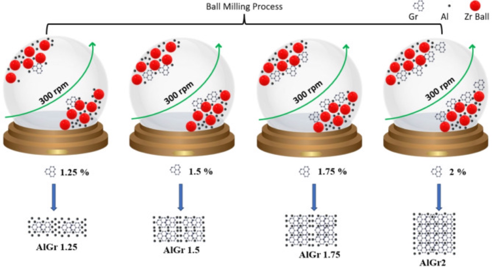
The researchers had already measured emission from pure aluminium and from aluminium containing 0.5 and 1.0 per cent graphene by weight. They set out to estimate what the emission behaviour would look like at higher graphene contents, at 1.25, 1.5, 1.75 and 2.0 per cent by weight, without making and testing those samples.

Where AI came in

The AI here is a set of statistical prediction models trained on the earlier measurements. Current-density-against-field data and current-stability data for the three measured compositions were merged into one table of four quantities: electric field, current density, emission current and time. The figures were rescaled to a common range and stray outliers removed. Models from five families were then fitted, including decision-tree methods, support vector regression, two small neural networks, Gaussian process regression and polynomial fitting. Each was scored by how well it reproduced data held back during training, and the best of each family was carried forward into a second round using gradient-boosting methods and combinations of models.

The combined, or stacked, model was then asked for compositions outside the range it had been trained on. Its outputs are the emission curves, stability traces, Fowler–Nordheim plots and turn-on fields reported for 1.25 to 2.0 per cent graphene. The best-scoring model reached an R² of 0.936577 and an RMSE of 10.28766 under ten-fold cross-validation, and the predicted turn-on field fell from 1.81 to 1.47 volts per micrometre across that range. In other words, the model stood in for the laboratory work of making and testing those four composites, and the paper states that these above-1 per cent results have not been checked against experiment.

Written by AIxSci from the checked record below, to give context for readers outside the field. It is not part of the record.

The work

Technical · from the record

The authors fitted regression models to previously measured field emission data for pure aluminium and aluminium composites with 0.5 wt% and 1.0 wt% graphene, then used the fitted models to produce emission current density versus electric field curves, current stability traces and Fowler–Nordheim plots for compositions with 1.25, 1.5, 1.75 and 2.0 wt% graphene, for which no measurements were available. A stacking ensemble of gradient-boosted models gave the lowest reported error, with R² of 0.936577 and RMSE of 10.28766 under 10-fold cross-validation. The predicted turn-on field at J = 10 µA cm−2 fell from 1.81 V µm−1 for 1.25 wt% to 1.47 V µm−1 for 2.0 wt% graphene. The paper states that these above-1 wt% outputs remain unverified by experiment.

How AI was used

Experimental current-density-versus-electric-field data (65 points per composition) and current-stability data (1800 points per composition) for pure aluminium, AlGr0.5 and AlGr1.0, taken from the authors' earlier work, were merged into a single table of four variables: electric field, current density, emission current and time. The data were Min-Max normalised and outliers in the emission current were removed using the interquartile range method. Two regression set-ups were defined, one predicting emission stability from current density, field and time, the other predicting current density from field, time and stability. In Stage 1, models from five families were fitted with largely default hyperparameters: Random Forest, Extra Trees and Decision Tree; SVR and Nu-SVR with an RBF kernel; an MLP and a TensorFlow Keras feedforward network with two 64-neuron hidden layers; Gaussian Process Regression and Bayesian Ridge; and third-degree polynomial regression, Monte Carlo bootstrap resampling and Holt-Winters smoothing. Models were ranked by MSE, RMSE, R² and Adjusted R² under 5-fold and 10-fold cross-validation with random_state = 42, and the best model from each family was carried into Stage 2, where XGBoost, LightGBM and CatBoost (n_estimators = 500, learning_rate = 0.01, max_depth = 7) and stacking, voting and bagging ensembles were fitted. The resulting models were then run at graphene loadings of 1.25, 1.5, 1.75 and 2.0 wt%, outside the range of the training data.

The shape of the work

Structural · the record, drawn

AI stepNo AI↤ what the AI stood in for

1Experiment
no AI

Synthesise aluminium–graphene composites

Physical execution, by hand or by robot.

High-energy ball milling (HBM) was performed at a rotational speed of 300 rpm for 10 hwhere the paper describes this · verbatim

in the paper

2Acquisition
no AI

Obtain field emission datasets from prior experimental work

Obtaining raw data, whether by measurement, download or retrieval.

the raw experimental data used to generate these structured datasets were sourced directly from our previous workwhere the paper describes this · verbatim

in the paper

3Preparation
no AI

Merge, normalise and clean training data

Cleaning, filtering, normalising or labelling data already obtained.

Prior to training, all data were subjected to normalization using the Min-Max scaling methodwhere the paper describes this · verbatim

in the paper

4Training
AI

Stage 1: train five baskets of regression models

Fitting model parameters, including fine-tuning an existing model.

In the stage 1, the models were trained using the experimental dataset consisting of pure Aluminum, 0.5 wt% of graphene inside Aluminium matrixwhere the paper describes this · verbatim

in the paper

5Validation
no AI

Score models and select best per basket

Testing outputs against ground truth.

The best-performing model from each category was selected for further refinement in the stage 2where the paper describes this · verbatim

in the paper

6Training
AI

Stage 2: refine with boosting and ensembles

Fitting model parameters, including fine-tuning an existing model.

Ensemble learning techniques, such as Stacking, Voting, and Bagging, were incorporated to enhance model robustness by combining multiple predictionswhere the paper describes this · verbatim

in the paper

7Inference
AI

Predict emission behaviour for 1.25–2.0 wt% graphene

Running a trained model over new data to predict, classify or score. The AI stood in for physical experiment.

The trained models were applied to aluminum composites with graphene weight percentages of 1.25 wt%, 1.5 wt%, 1.75 wt%, and 2.0 wt%where the paper describes this · verbatim

in the paper

8Validation
no AI

Check predictions against expected trends and reported values

Testing outputs against ground truth.

By comparing the predicted field emission characteristics at these higher graphene concentrations with expected trendswhere the paper describes this · verbatim

in the paper

What the record says

Technical · every part carries its own basis

+ in the paper~ our reading− not reported

How to read the quotations. A quotation shows where the paper describes something. It does not quote every value beside it: one passage locates a part of the work, and values without their own quotation are our reading of that passage.

~Role of AI

AI produced the resultour reading

The reported field emission curves, Fowler–Nordheim plots and turn-on fields for 1.25–2.0 wt% graphene are model outputs; no measurement exists for those compositions in this paper

+What the AI was for

Property predictionin the paper

Bayesian Models, including Gaussian Process Regressor (GPR) and Bayesian Ridge were introduced to incorporate probabilistic approacheswhere the paper describes this · verbatim

+Model families

Gaussian process Support vector machine Random forest Gradient-boosted trees Multilayer perceptron Linear modelin the paper

+How it was taught

Supervisedin the paper

+Models named

Gaussian Process Regressor (GPR) · Trained from scratchSupport Vector Regression (SVR) · Trained from scratchNu-SVR · Trained from scratchRandom Forest Regressor · Trained from scratchExtra Trees · Trained from scratchDecision Tree · Trained from scratchMulti-Layer Perceptron (MLP) · Trained from scratchFeedforward Neural Network (FNN, TensorFlow Keras) · Trained from scratchBayesian Ridge Regression · Trained from scratch3rd-degree Polynomial Regression · Trained from scratchMonte Carlo bootstrap with Random Forest base estimator · Trained from scratchHolt-Winters Exponential Smoothing · Trained from scratchXGBoost · Trained from scratchLightGBM · Trained from scratchCatBoost · Trained from scratchStacking ensemble (XGBoost, LightGBM, CatBoost with Ridge final estimator) · Trained from scratchVoting ensemble · Trained from scratchBagging ensemble · Trained from scratchin the paper

+How results were checked

Held-outin the paper

both 5-fold and 10-fold cross-validation strategies were employed during training and performance assessmentwhere the paper describes this · verbatim

+Code · weights · data

code not reportedweights not reporteddata not availablein the paper

the paper does not include the full dataset in tabular formwhere the paper describes this · verbatim

+Compute

not reportedin the paper

What this paper did not report

Technical · absence is published deliberately

Reported as not stated — 24 items

CodeWhether the code is available is not stated.
Trained model weightsWhether the trained model is available is not stated.
ComputeThe hardware or time used is not stated.
How many were testedThe paper gives no count of what was tested.
Version of Gaussian Process Regressor (GPR)Which version of the model was used is not stated.
Version of Support Vector Regression (SVR)Which version of the model was used is not stated.
Version of Nu-SVRWhich version of the model was used is not stated.
Version of Random Forest RegressorWhich version of the model was used is not stated.
Version of Extra TreesWhich version of the model was used is not stated.
Version of Decision TreeWhich version of the model was used is not stated.
Version of Multi-Layer Perceptron (MLP)Which version of the model was used is not stated.
Version of Feedforward Neural Network (FNN, TensorFlow Keras)Which version of the model was used is not stated.
Version of Bayesian Ridge RegressionWhich version of the model was used is not stated.
Version of 3rd-degree Polynomial RegressionWhich version of the model was used is not stated.
Version of Monte Carlo bootstrap with Random Forest base estimatorWhich version of the model was used is not stated.
Version of Holt-Winters Exponential SmoothingWhich version of the model was used is not stated.
Version of XGBoostWhich version of the model was used is not stated.
Version of LightGBMWhich version of the model was used is not stated.
Version of CatBoostWhich version of the model was used is not stated.
Version of Stacking ensemble (XGBoost, LightGBM, CatBoost with Ridge final estimator)Which version of the model was used is not stated.
Version of Voting ensembleWhich version of the model was used is not stated.
Version of Bagging ensembleWhich version of the model was used is not stated.
What step 4 replacedThe paper gives no basis for what the AI stood in for.
What step 6 replacedThe paper gives no basis for what the AI stood in for.

About this article

Record aix-00133, version 2, checked by a person on 2026-10-09. The record describes the paper; it does not assess whether the paper's findings are right. The paper is published under CC-BY; quotations are at most 25 words. How we work · Report an error