materials-chemistry/ai produced the result/ACS Omega 2023 · v2
Neural networks predict how much ultrasound energy drives magnesia dissolution
Researchers dissolved calcined magnesite ore in carbonated water while applying ultrasound, then trained small neural networks on the resulting measurements to predict the fraction of ultrasound energy converted in the reaction.
spectrum · one line per step, placed by what the step does · bright lines used AI
Artificial Neural Network Approach for Modeling of Effect of Ultrasound on the Dissolution of Magnesia in Aqueous Carbon Dioxide
ACS Omega, 2023
doi:10.1021/acsomega.3c03668 · record aix-00213 v2 · checked 2026-10-09
- AI was for
- Property prediction
- Model family
- Multilayer perceptron
- Checked by
- Held-out
- Code
- not reported
The finding the paper is about came from the AI.
What this research was about
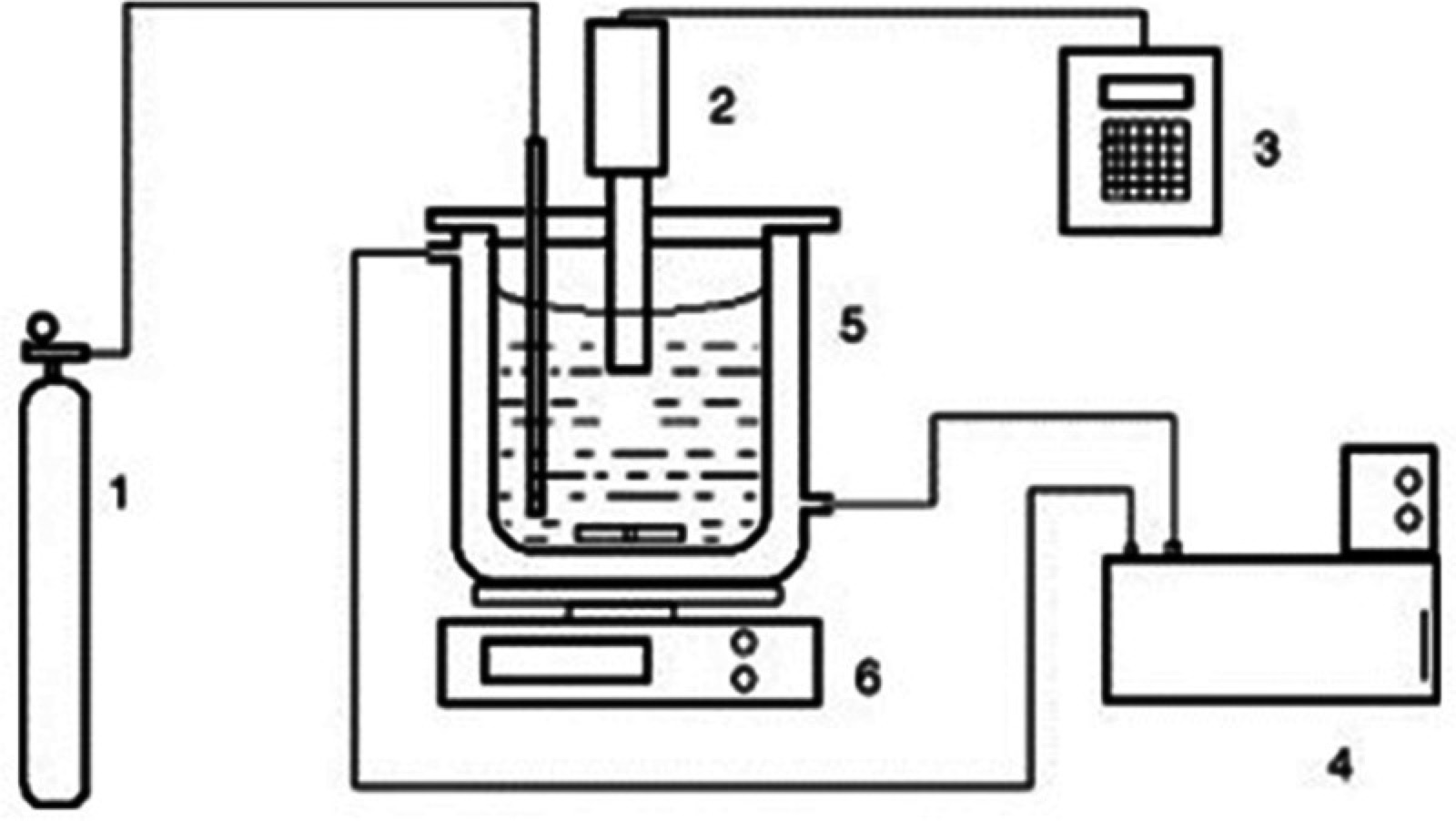
Magnesite is a mineral rich in magnesium carbonate. Heating it drives off carbon dioxide and leaves magnesia, a magnesium oxide powder. To recover the magnesium in a useful form, chemists dissolve that powder in water charged with carbon dioxide, a process known as leaching. How fast it dissolves depends on several things at once: how finely the powder is ground, how warm the liquid is, how much solid there is for a given volume of liquid, and how long the reaction runs. Adding ultrasound stirs and agitates the liquid at a very small scale, which can speed dissolution, but only part of the energy sent into the vessel actually does useful work.
The researchers ran leaching experiments on magnesite ore that had been crushed, sieved and calcined, dissolving it in carbon-dioxide-saturated distilled water in a jacketed glass reactor fitted with an ultrasonic probe. They varied particle size, temperature, the solid-to-liquid ratio and the ultrasound amplitude, and tracked the magnesium released over time. Separately they measured how much power the ultrasound device delivered, using the temperature rise of insulated water and a chemical test, which let them work out what they call the ultrasound energy conversion fraction for each setting.
Where AI came in
The artificial neural network came in after the laboratory work. A network of this kind is a mathematical function with adjustable internal numbers, tuned until it reproduces a set of examples; here the examples were the team's own measurements. Five quantities were fed in — particle size, time, reaction temperature, solid-to-liquid ratio and amplitude rate — and the network returned a single value, the ultrasound energy conversion fraction. The 110 records were split at random into seventy per cent for fitting the network, fifteen per cent for checking progress during fitting and fifteen per cent held back entirely for testing.
Six networks were built in MATLAB's neural network toolbox, pairing two fitting algorithms, Levenberg–Marquardt and gradient descent, with three internal response functions. The number of units in the network's hidden middle layer was searched between three and twenty, and different starting values were tried. The trained networks' predictions were then compared with the measured values to pick the best; Levenberg–Marquardt with the TANSIG function agreed most closely, with a reported regression R of 0.99 for both the training and the test data. The network stands in for an explicit formula relating the reaction conditions to the energy fraction.
Written by AIxSci from the checked record below, to give context for readers outside the field. It is not part of the record.
The work
Technical · from the record
Magnesia from calcined magnesite ore was dissolved in CO2-saturated water under ultrasound, with particle size, reaction temperature and solid/liquid ratio varied, and the ultrasound energy conversion fraction (USECF) was obtained from the experiments. The experimental data were then used to fit artificial neural networks that predict USECF from particle size, time, reaction temperature, solid/liquid ratio and amplitude rate. Six networks were built from two learning algorithms and three transfer functions and their outputs compared with the experimental values; the Levenberg–Marquardt algorithm with the TANSIG transfer function gave the closest agreement, and Gradient Descent with LOGSIG was second. Regression R was reported as 0.99 for the training data after validation and 0.99 for the test data.
How AI was used
The authors used the measurements from their own leaching experiments as the training material for feed-forward multilayer perceptron networks implemented in the MATLAB R2018b neural network toolbox. Five experimental variables — particle size, time, reaction temperature, solid/liquid ratio and amplitude rate — were taken as inputs and the ultrasound energy conversion fraction as the single output, with the original unnormalised values used directly. The 110-record data set was split randomly into 70% training, 15% validation and 15% test data. Six networks were trained, combining the Levenberg–Marquardt and Gradient Descent back-propagation algorithms with the TANSIG, PURELIN and LOGSIG transfer functions, while the number of hidden-layer neurons was searched between 3 and 20 and different initial weighting coefficients were tried; the paper reports the best result being reached at 20 000 iterations. The trained networks were then run to predict USECF, and mean squared error and regression R against the experimental targets were used to choose among the architectures.
The shape of the work
Structural · the record, drawn
no AI
Calcine ore and run ultrasound-assisted leaching experiments
Physical execution, by hand or by robot.
a 2.0 g sample of magnesia was added and stirred mechanicallywhere the paper describes this · verbatim
no AI
Determine ultrasound power and energy conversion fraction
Obtaining raw data, whether by measurement, download or retrieval.
the power of the ultrasound device was determined using the calorimetric method and the Weissler reactionwhere the paper describes this · verbatim
no AI
Assemble data set and split train/validation/test
Cleaning, filtering, normalising or labelling data already obtained.
All experimental data were divided randomly into three groups, i.e., training (70%), validation (15%), and testing data (15%).where the paper describes this · verbatim
AI
Train six ANN models
Fitting model parameters, including fine-tuning an existing model.
Levenberg–Marquardt and Gradient Descent learning algorithms were used to create ANN modelswhere the paper describes this · verbatim
AI
Search hidden-layer size and transfer function
Iterative search over a space. Its result feeds back into an earlier step.
The number of neurons was optimized between 3 and 20 neurons in the hidden layerwhere the paper describes this · verbatim
AI
Predict USECF with trained models
Running a trained model over new data to predict, classify or score.
USECF was determined as the output variable of the model.where the paper describes this · verbatim
no AI
Compare predictions with experimental values and pick best model
Testing outputs against ground truth.
Correlation coefficients for training, validation, and test data were determined as 0.99, 0.99, and 0.99, respectively.where the paper describes this · verbatim
What the record says
Technical · every part carries its own basis
+ in the paper~ our reading− not reported
How to read the quotations. A quotation shows where the paper describes something. It does not quote every value beside it: one passage locates a part of the work, and values without their own quotation are our reading of that passage.
The paper has two stages: leaching experiments, then an ANN model of the ultrasound energy conversion fraction. The reported modelling result (regression R values) exists only because of the neural network, so the second stage's claim is produced by the model. The dissolution observations themselves do not depend on it, so 'analysis' is a defensible alternative reading.
ANN modeling of multilayer perceptron with Gradient Descent and Levenberg–Marquardt algorithmswhere the paper describes this · verbatim
The test data set is not used in training at allwhere the paper describes this · verbatim
an artificial neural network model was created in accordance with this data set (Appendix 1)where the paper describes this · verbatim
What this paper did not report
Technical · absence is published deliberately
- CodeWhether the code is available is not stated.
- Trained model weightsWhether the trained model is available is not stated.
- ComputeThe hardware or time used is not stated.
- How many were testedThe paper gives no count of what was tested.
- Version of Multilayer perceptron ANN, Levenberg–Marquardt with TANSIG transfer function (LM1)Which version of the model was used is not stated.
- Version of Multilayer perceptron ANN, Gradient Descent with LOGSIG transfer function (GD3)Which version of the model was used is not stated.
- What step 4 replacedThe paper gives no basis for what the AI stood in for.
- What step 5 replacedThe paper gives no basis for what the AI stood in for.
- What step 6 replacedThe paper gives no basis for what the AI stood in for.
About this article
Record aix-00213, version 2, checked by a person on 2026-10-09. The record describes the paper; it does not assess whether the paper's findings are right. The paper is published under CC-BY; quotations are at most 25 words. How we work · Report an error